Global Warming and Data Science, Episode 2: Data Engineering and Loading into Snowflake

In the previous episode, I discussed the goals of my current work side-project: loading a fairly sizable weather data set from NOAA and analyzing is using data science techniques and machine learning.

This post will get into the nitty-gritty of how I went ahead and massaged (‘wrangled’) the data into a form Snowflake finds palatable to digest and load into tables from text/CSV files. Subsequent posts will go into the specifics of the analytics. This is all about the dark art of data engineering. I am not a pro data engineer and many are lucky to have their own tools, so take this with a view of me as a dangerous neophyte.

The dataset I am using is officially named ‘Global Historical Climatology Network – Daily‘, or GHCND to its friends. It comes in two flavors:

1. Data arranged per location (weather station), with each row containing a pre-set collection of data points (high/low temperature, wind speed, precipitation, etc.) for one day.
2. Super GHCND – each row contains one data point about one weather station on one day.

The Super GHCND dataset involves a 100GB download of a daily-updated, all-station-history-data file called superghcnd_full_<creation date>.csv.gz (e.g. superghcnd_full_20180905.csv.gz) from here, along with several metadata files:

• ghcnd-countries – the list of country codes
• ghcnd-states – a list of states and provinces
• ghcnd-stations – the weather station names, codes, and location information
• ghcnd-inventory – inventory listing the availability of data points for each weather station. For examples, a station may offer daily high and low temperatures from 1929 to the current day but wind speed is only available from 1944.

Data Engineering in Domino

Before we get the files into Snowflake, we need to download them and adapt them to the format that would work for its data loading functions. The process will look like this:

1. Download the files
2. Adapt them to a CSV or another character-delimited file (because commas don’t work in all situations, sadly)
3. Upload the file into Snowflake using the Snowsql tool
4. Use Snowsql to load the files into database tables we can use for our work

Big data in Domino? use Domino Datasets!

If you are about to download a large file in the hundreds of megabyte size range or larger, or have a vast number of data files to process, Domino recommends you use your project’s Dataset facility instead of files. Besides a clean separation between your code and data, datasets allow Domino to optimize file storage, sharing and the way they are loaded into your environment.

Since our first file starts out at 11GB, we will use a dataset!

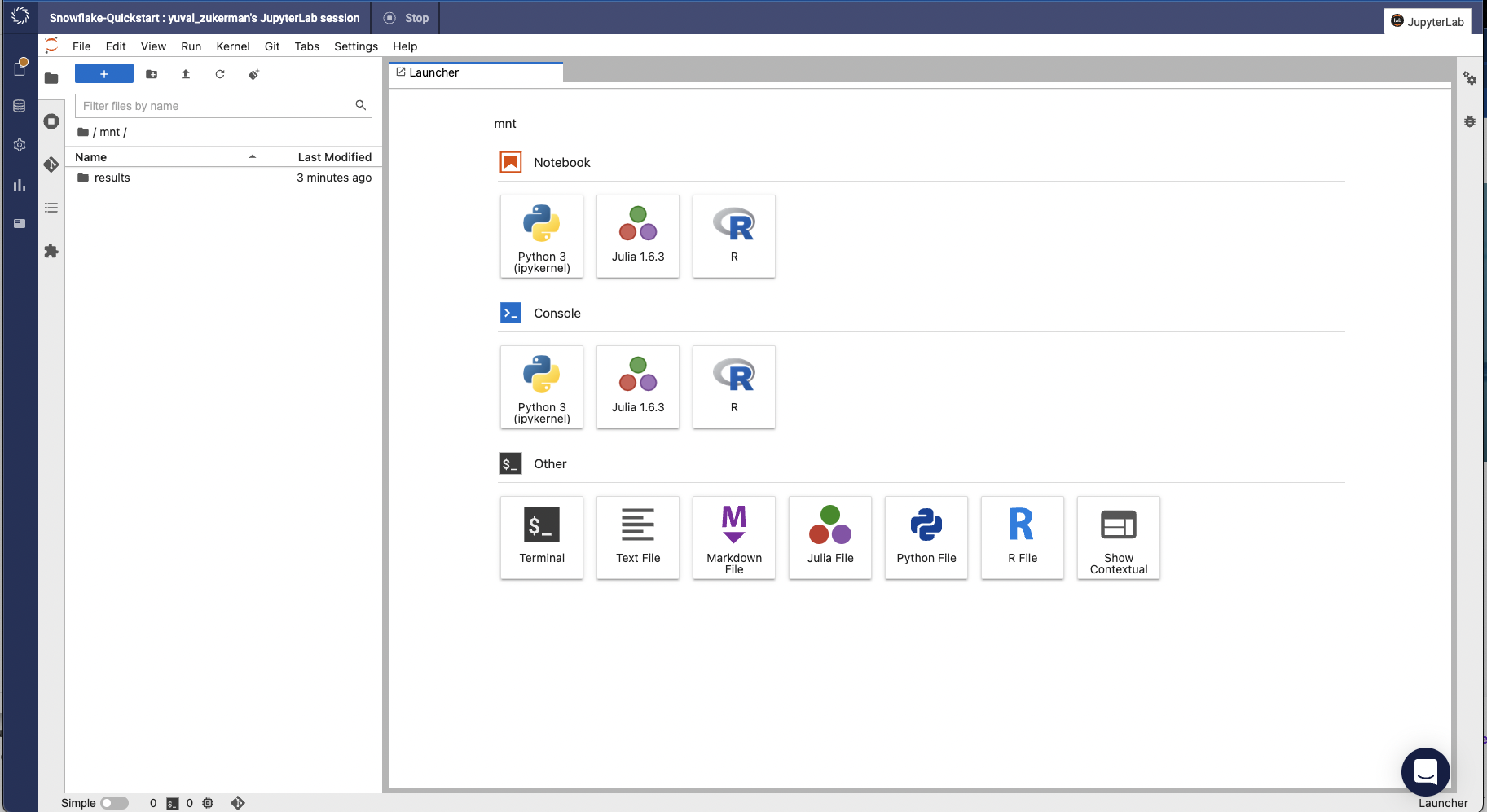
If you haven’t done so already, log into Domino and create a new project. I called my project ‘Snowflake-Quickstart’. Then, open a new workspace, normally the Domino default environment with Python, and choosing JupyterLab as your IDE. It should look something like this:

Once you click ‘Launch’, a new browser tab will open and your workspace will start loading. After a minute or two – depending on the availability of resources in your Domino environment – the workspace will open and you should see something like this:

The final step is to start a Terminal, which will allow us to access and manipulate our data files using Linux’s built-in file processing tools.

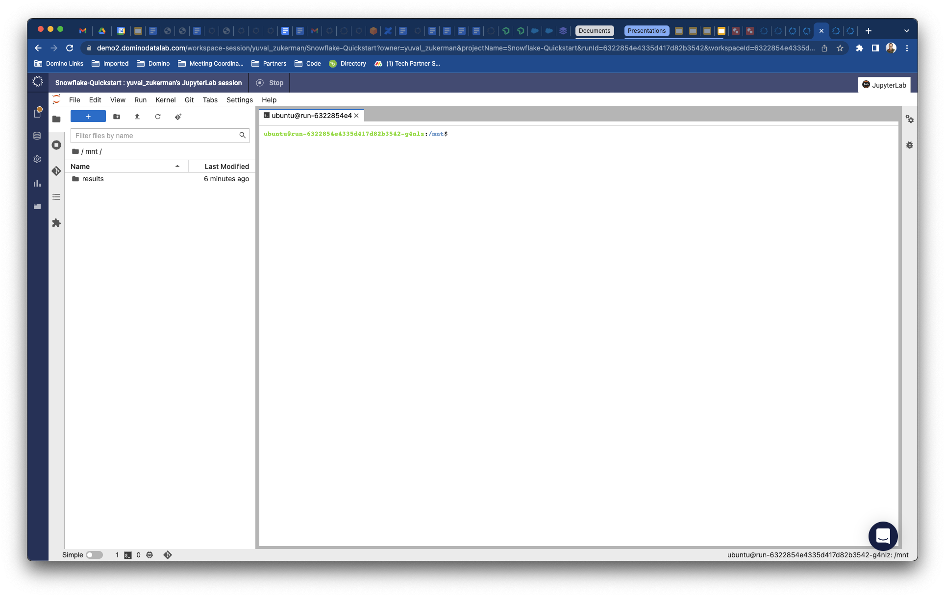
Domino’s datasets reside in a special directory:

/domino/datasets/local/<project name>/
Code language: HTML, XML (xml)

Let’s switch to that directory for the time being:

cd /domino/datasets/local/<project name>/
Code language: HTML, XML (xml)

In our case, that will be /domino/datasets/local/Snowflake-Quickstart/. We will use the wget command to download the files. To download the files listed above… (bold used to highlight the filename)

wget https://www.ncei.noaa.gov/pub/data/ghcn/daily/<strong>ghcnd-stations.txt</strong> 

wget https://www.ncei.noaa.gov/pub/data/ghcn/daily/<strong>ghcnd-countries.txt</strong> 

wget https://www.ncei.noaa.gov/pub/data/ghcn/daily/<strong>ghcnd-states.txt</strong>

wget https://www.ncei.noaa.gov/pub/data/ghcn/daily/<strong>ghcnd-inventory.txt</strong> 

wget https://www.ncei.noaa.gov/pub/data/ghcn/daily/superghcnd/<strong>superghcnd_full_<date of newest file>.csv.gz </strong>
Code language: Bash (bash)

We should now start unzipping the large superghcnd_full_ file using the command:

gunzip superghcnd_full_<date>.csv.gz
Code language: CSS (css)

Depending on the Domino instance you are using, this extraction can take a while. You can add an ampersand to the end of the line, which will run the command in the background.

File Formatting

While the main data file is a ‘proper’ CSV file, these metadata files use size-delimited fields. For example:

------------------------------
Variable   Columns   Type
------------------------------
ID            1-11   Character
LATITUDE     13-20   Real
LONGITUDE    22-30   Real
ELEMENT      32-35   Character
FIRSTYEAR    37-40   Integer
LASTYEAR     42-45   Integer
------------------------------

What this looks like in practice is something like this:

ACW00011647  17.1333  -61.7833 WT16 1961 1966
AFM00040990  31.5000   65.8500 TAVG 1973 2020
AG000060390  36.7167    3.2500 TMAX 1940 2022
Code language: CSS (css)

I could not figure out how to load these into Snowflake (supported formats do not include field size-based data), so I turned to regular expressions and classic Unix utilities, sed and tr. Sed is especially great because it is a stream editor – it reads chunks, normally lines, and is able to modify each line independent of the next. In general, Sed works in a nifty way when using (truly basic) regular expressions:

sed 's/<pattern to match>/<replacement text>/<location in the line or everywhere>' > <output file>
Code language: HTML, XML (xml)

While I am sure there is more than one way to do it, I stuck with Sed and used command lines like these:

sed 's/./|/12;s/./|/21;s/./|/31;s/./|/38;s/./|/41;s/./|/72;s/./|/76;s/./|/80' ghcnd-stations.txt > ghcnd-stations.csv
Code language: JavaScript (javascript)

Deconstructed:

• Looking at the first replacement in the line:

s/./|/12

That would mean: “Count 12 characters that mach the regular expression ‘.’ – any character – and put the character ‘|’ (vertical bar) there.

I repeat such directives throughout the line, separated by semicolons, to place vertical bar characters to delimit between the fields. The outcome will look this:

ACW00011647|17.1333|-61.7833|WT16|1961|1966
AFM00040990|31.5000|65.8500|TAVG|1973|2020
AG000060390|36.7167|3.2500|TMAX|1940|2022

You note that I used a vertical bar as the delimiter. It appears some data in the files has commas, which can add ‘columns’ to the file unintentionally. While suboptimal (the vertical bar is a Unix operand), it will make do for our project.

Similarly, we will convert the inventory and country files using:

sed 's/./|/12;s/./|/21;s/./|/31;s/./|/36;s/./|/41' ghcnd-inventory.txt > ghcnd-inventory.csv

sed 's/./|/3' ghcnd-countries.txt > ghcnd-countries.csv

sed 's/./|/3' ghcnd-states.txt > ghcnd-states.csv
Code language: JavaScript (javascript)

Collecting a data subset

While in the real world data sets as big as 100GB are reasonable, to simplify matters we will extract a subset of this data, around 2GB, with weather information for Western Europe. The reason is that Western Europe had consistently collected weather data over the last 70 years or so. These countries include:

• Germany (mostly West Germany)
• Italy
• France
• Spain
• UK
• Portugal
• The Netherlands
• Belgium
• Switzerland
• Austria

Since each entry in the data set represents one data item for a weather station, it starts with the weather station’s ID. That ID starts with the country code, so we can filter the data set to give us just the information we need, for these countries.

We will again use the Sed tool to pick up these countries’ identifying country code so we can pick the data up from the big data set we unzipped. One way is to ask about one country, get the country code, and extract its data from the full data set into a file. That will look like:

% sed -n '/Neth.*/p'
Code language: JavaScript (javascript)

Which will return the code for The Netherlands:
NL Netherlands

Instead we will try to abbreviate into this:

% sed -n '/Neth.*/p;/Ita*/p;/Spa*/p;/.. United K.*/p;/Germany/p;/Switz*/p;/Portu*/p;/Belg.*/p;/.. France/p;/Austria/p' ghcnd-countries.txt
AU Austria 
BE Belgium 
FR France 
GM Germany 
IT Italy 
NL Netherlands 
PO Portugal 
SP Spain 
SZ Switzerland 
UK United Kingdom 
Code language: JavaScript (javascript)

And now, to extract the data from the dataset, we can do that for one country like this:

% sed -n '/^NL.*/p' superghcnd_full_20220907.csv > netherlands_data.csv
Code language: JavaScript (javascript)

To break it down:

• -n – Suppress output
• /^NL.* – Return lines starting with NL (^) followed by any number of characters
• /p – prints the line

We then redirect the output to a new file.
So now we are going to combine all these statements, for all the countries on our lies, using the codes we extracted, into one command:

sed -n '/^AU.*/p;/^BE.*/p;/^FR.*/p;/^GM.*/p;/^IT.*/p;/^NL.*/p;/^PO.*/p;/^SP.*/p;/^SZ.*/p;/^UK.*/p' superghcnd_full_<strong><your file date></strong>.csv > west_euro_data.csv
Code language: HTML, XML (xml)

The result will be just under 4GB. For in-person on online workshops we will refine this further to the last 50 years and to stations that are still functioning throughout that time.

We can use the identical treatment on the weather station and station inventory files:

sed -n '/^AU.*/p;/^BE.*/p;/^FR.*/p;/^GM.*/p;/^IT.*/p;/^NL.*/p;/^PO.*/p;/^SP.*/p;/^SZ.*/p;/^UK.*/p' ghcnd-stations.csv > ghcnd-stations-west-eu.csv

sed -n '/^AU.*/p;/^BE.*/p;/^FR.*/p;/^GM.*/p;/^IT.*/p;/^NL.*/p;/^PO.*/p;/^SP.*/p;/^SZ.*/p;/^UK.*/p' ghcnd-inventory.csv > ghcnd-inventory-west-eu.csv
Code language: Bash (bash)

At this point we are finally ready to go Snowflake!

Data Loading into Snowflake

Data is loaded into Snowflake by staging: that means uploading the data to a special area in your Snowflake account OR telling Snowflake to pull your data from an AWS or Azure data store. I’m low-brow, and chose the local file-to-stage route, which means uploads.

If you, like me, had never used Snowflake, the first step is to download Snowflake’s rather nifty command line interface admin tool, Snowsql. Domino offers a Snowflake-optimized environment that has the tool preinstalled. All you will need to connect is your account ID, username and password, along with the names of your warehouse, database and schema (which is often ‘PUBLIC’). Once connected you will be presented with an interface to your very own cloud database. The fastest way to connect will be to connect using command-line options, such as:

snowsql -a <account ID> -u <user name> -w <warehouse name> -d <database name> -s <schema name> -o log_file=~/.snowsql/log
Code language: HTML, XML (xml)

You will be prompted to enter your password once connected. The following steps are all executed in Snowsql.

Before we upload the data, we need to define tables to hold the data. This is how it looks in an entity-relationship diagram:

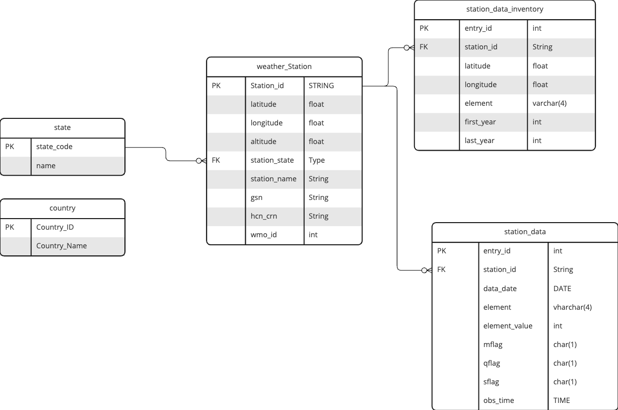
The corresponding SQL file is available here.

Download and open the file and run it, command by command in snowsql.

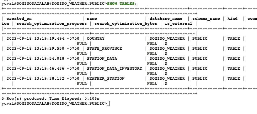
When you are done, you should see the tables like this when you run the command
show tables;

The following steps are based on Snowflake’s own snowsql data loading tutorial, which we will follow to upload the data we wrangled in the previous steps:

• Create a file format object – this helps guide Snowflake how to read your file and map it into your database tables. The provided example is:

create or replace file format bar_csv_format
  type = 'CSV'
  field_delimiter = '|'
  skip_header = 1;
Code language: SQL (Structured Query Language) (sql)

(yes ‘csv’ stands for comma-separated values and we our delimiter is ‘vertical bar’ so deal with it). We need to create another file format for our main data file, which uses commas as delimiters:

CREATE OR REPLACE FILE FORMAT comma_csv_format
type = 'CSV' field_delimiter = ',';
Code language: SQL (Structured Query Language) (sql)

• Next, we create the stage, the holding area for uploaded files and add our file format specification to it (we will use the other file format later):

create or replace stage weather_csv_stage
  file_format = bar_csv_format;
Code language: SQL (Structured Query Language) (sql)

• We can now upload the files from Domino. Make sure you adjust the command to the right directory for your dataset:

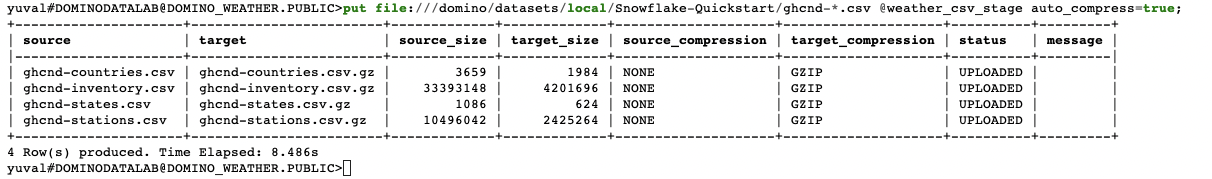
put file:///domino/datasets/local/<project dataset directory>/ghcnd*.csv @weather_csv_stage auto_compress=true;                                                                                  
Code language: HTML, XML (xml)

The result will look like this:

• You can also list the files you uploaded using the command:

list @weather_csv_stage;
Code language: CSS (css)

• Now, we will upload our Western European data file

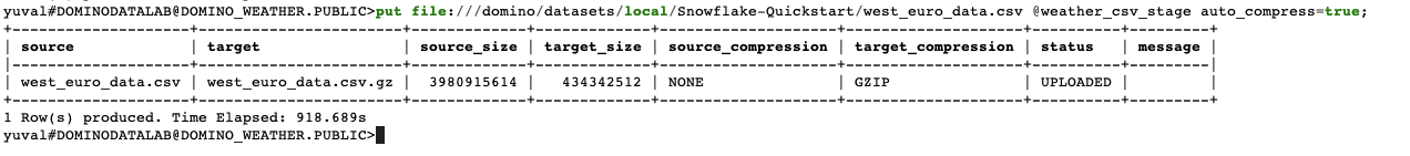
put file:///domino/datasets/local/<your project dataset directory>/west_euro_data.csv @weather_csv_stage auto_compress=true;
Code language: JavaScript (javascript)

This will take a while but eventually, the result should look something like this:

From data files into tables

We are finally ready to load the data into Snowflake database tables. That is done using the COPY INTO command, and we will start with the smaller files and ensure foreign key constraints are followed.

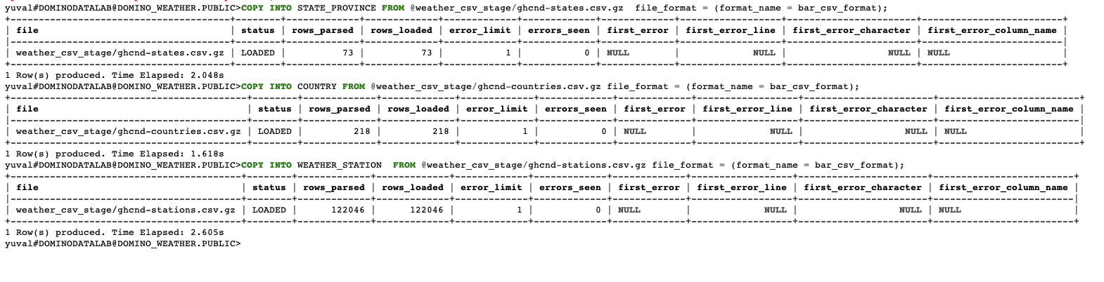
COPY INTO STATE_PROVINCE FROM @weather_csv_stage/ghcnd-states.csv.gz  file_format = (format_name = bar_csv_format);

COPY INTO COUNTRY FROM @weather_csv_stage/ghcnd-countries.csv.gz file_format = (format_name = bar_csv_format);

COPY INTO WEATHER_STATION FROM @weather_csv_stage/ghcnd-stations-west-eu.csv.gz file_format = (format_name = bar_csv_format);
Code language: SQL (Structured Query Language) (sql)

These are relatively straight-forward and should result in something like this:

The station data inventory is slightly more complex:
We are using an artificial identity field as primary key so need to load data from the csv file into specific columns. This is done using a subquery, resulting in something that looks like this:

COPY INTO station_data_inventory
(station_id, latitude, longitude, element, first_year, last_year) 
FROM
(select t.$1, t.$2, t.$3, t.$4, t.$5, t.$6
from @weather_csv_stage
(file_format => 'bar_csv_format', 
pattern => '.*ghcnd-inventory-west-eu.csv.gz') t)
ON_ERROR = CONTINUE;
Code language: SQL (Structured Query Language) (sql)

This will result in hundreds of thousands of rows being loaded – Snowflake will show you how many were ready in the result. Note that we are using the ‘ON_ERROR = CONTINUE’ behavior as in very large data files, errors can occur and we can tolerate missing a small number of row.

Finally, we will load the Western Europe dataset in similar fashion:

COPY INTO STATION_DATA 
(STATION_ID, DATA_DATE, ELEMENT, ELEMENT_VALUE, MFLAG, QFLAG, SFLAG, OBS_TIME)
FROM
(select 
t.$1, TO_DATE(t.$2, 'yyyymmdd'), t.$3, t.$4, t.$5, t.$6, t.$7, TO_TIME(t.$8, 'hhmm') 
from @weather_csv_stage 
(file_format => 'COMMA_CSV_FORMAT', 
pattern => '.*west_euro_data.csv.gz') t)
ON_ERROR = CONTINUE;
Code language: SQL (Structured Query Language) (sql)

We will have approximately 120 million rows of data. Just to show you just how fast Snowflake is, try running this query that will count how many unique station IDs exist in this large table :

SELECT COUNT(DISTINCT STATION_ID) AS STATION_COUNT FROM STATION_DATA;
Code language: PHP (php)

Impressed?

The next episode will focus on whittling down the data – this time in Domino – with Snowflake code.